Personal tools
Gnuplot and Gnufit
GnuPlot
This is a brief introduction to GnuPlot. There is also the original user's manual available on-line.
To start gnuplot in UNIX type
gnuplot
and the prompt gnuplot> will appear on the screen.
Gnuplot has a hierarchical help system. It displays the requested information screen-wise (press Enter to get to the next page) and then usually displays a list of sub-items. You can then enter one of them to get information about it, or just press Enter to go back one level (or leave the help system).
You enter the help system by typing the command help, optionally
followed by a command name, if you already know what you're looking for.
Having worked through the very basic examples presented here, you should
take a closer look at the many options Gnuplot offers.
You can plot a function using the plot command:
plot sin(x)
To specify the plot range, write:
plot [x=-10:10] sin(x)
To overlay two function plots:
plot [x=-10:10] sin(x),cos(x)
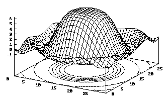
Use the splot command:
   set contour
   set hidden3d
   splot [-pi:pi] [-pi:pi] sin(x*x+y*y)/(x*x+y*y)

To alter the view point type, for example
set view 75, 60, 1, 1
It rotates about the screen horizontal axis by 75 degrees, about the screen vertical by 60 degrees, and scales the x and y directions by unity.
To strip off the labeling detail use, e.g.,
   set noborder
   set nokey
   set nolabel
   set noxzeroaxis
   set noyzeroaxis
   set noxtics
   set noyticks
   set nozticks
You can also plot numerical data saved in a text file. Gnuplot expects one data point per line. Lines that start with the hash symbol (#) are ignored. Empty lines mark the end of one graph and the beginning of the next.
For instance, let's assume that you have a data file called xy.dat looking like:
   # my experimental data
   #  X     Y
     1.0   1.3
     2.1   4.2
     3.0   9.5
To plot the data, write:
plot 'xy.dat' with lines
If you omit with lines, Gnuplot will not connect the data points.
Three dimensional data on the other hand must be saved in a different form:
   x1
   y1
   z1

   x2
   y2
   z2

   x3
   y3
   z3
Use the commands
        set noparametric
        set contour
        set hidden3d
        splot "datafile.dat" with lines
To have a contour plot, write
        set contour
        set nosurface
        set view 0, 0, 1, 1
  set title "plot of ..."      places a title above the plot box
  set nokey                    removes the plot key (6)
  set xlabel "argument ..."
  set ylabel "function ..."    ylabel titles rotates to
                                                  vertical under postscript
  set size  0.5, 0.5          for scaling the x and y directions
  set logscale x               to set Log scaling
  set samples  1000        More resolution (beyond the
                                         default of 160) is gained with.(7)
When you begin to use a lot of options, it is a good idea to save the
commands in a text file and load them from there with the load
command. This saves you the trouble of re-entering everything when you
want to make small modifications to the output.
If Gnuplot doesn't offer you all the features you are looking for, try Mathematica (see section Mathematica).
If you want to print the output, create a PostScript file first:
   set terminal postscript
   set output "output.ps"
   replot
From outside Gnuplot (either quit or open another terminal window), send the file to the printer:
lpr -Pprintername output.ps
If you want to include the output in a LaTeX document, create an EPS file instead:
   set terminal postscript eps
   set output "figure.eps"
   replot
See section Including figures in Latex on how to proceed.
GNUFIT is a nonlinear least squares fit mechanism into gnuplot.
It incorporates a nonlinear least squares fit mechanism into
gnuplot. The
fit uses the Marquardt-Levenberg-algorithm for fitting and the gnuplot
function evaluation mechanism for calculation.
It may fit every user-defined function to any set of data pairs (x,y). Note that (x,y) and the function's return type MUST be real!
Any variable occuring in the function body may serve as fit parameter (fitting functions without adjustable parameters make no sense).
Using GNUFIT
You must have
- a text file with data points as could be used for 2D plotting (see section Plotting Data),
- a function in x with parameters that will be modified in order
to make the function fit the data, e.g.
f(x) = exp(a1*x) * (a2*cos(a3*x) + a4*sin(a2*x))
- a text file that contains the initial values for the paramters:
  a1 = 1
  a2 = 1
  a3 = 1
  a4 = 1
The syntax would then be
fit f(x) 'datafile' via 'parameter file'
Special gnuplot variables:
- FIT_INDEX: This variable always contains the current data point number during execution starting with 1. You may use it in your fit function to implement multiple-branch-fits.
- FIT_SKIP: You may specify a positive integer to always skip i data points during fitting. This increases execution speed by the price of less exact results.
- FIT_LIMIT: may be specified to change the default epsilon limit (1e-5). When the sum of squared residuals changes between 2 iteration steps by less than a factor of this number, the fit is considered as 'converged'.
Example
    FIT_LIMIT = 1e-10
    FIT_SKIP = 2
    f(x)=exp(a1*x)*( a2*cos(a3*x) + a4*sin(a2*x) )
    fit f(x) 'Jo(x)-data' 'guess.a'
    #
    g(x)=b1+b2*x+b3*x**2+b4*x**3+b5*x**4+b6*x**5
    fit g(x) 'Jo(x)-data' 'guess.b'
    #
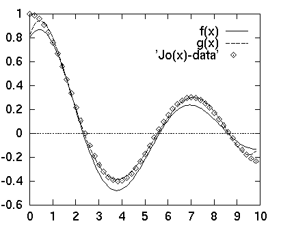
    plot f(x), g(x), 'Jo(x)-data'
would result in

In this example, two different analytical functions
(f(x) and g(x)) have
been used to fit the bessel function data set in the file "Jo(x)-data"
by starting the fitting with the guess parameter files "guess.a" for the
parameters a1, ..., a4
and "guess.b" for b1,..., b6.
The file "guess.a" should look like this:
             a1 = 1
             a2 = 1
             a3 = 1
             a4 = 1
update parameters
After the plot appeared in your graphics terminal (as in the figure above),
you may update the input
file 'guess.a' (containing the initial guess a1, a2, etc)
by simply typing
update "filename"
This command updates the start parameter assignments in a start parameter file (in the previous example this is guess.a). Each parameter will be replaced by its actual value. This is useful for restarting a converged or stopped fit again.
For example the update "guess.a" should now look like this
            a1              = -0.0826758
            a2              = 0.800099
            a3              = 0.955014
            a4              = 0.499098
Then repeat again the gnufit procedure for obtaining a new improved
fit of your data set (by simply loading the file containing the gnuplot
command as in the example of the previous subsubsection).
fit.log file
After each iteration step a detailed info is given about the fit's state both on the screen and on a so-called logfile
fit.log
This file will never be erased but always appended so that the fit's history isn't lost.